The basics of diffusion and perfusion imaging in brain tumors

Perfusion and diffusion magnetic resonance imaging (MRI) are commonly used by neuroradiologists in everyday clinical practice. These techniques provide information not available with conventional MRI. Response Assessment in Neuro-Oncology Criteria (RANO)¹ and Macdonald² criteria have been used extensively to evaluate tumor response based on measurement of T1 postcontrast images. However, relying on these changes can lead to misinterpretation of treatment response, since enhancement volume is a relatively nonspecific feature of tumor behavior.³

Perfusion and diffusion imaging are recent advances that can help predict tumor type and grade, as well as predict patient survival and optimal therapeutic options.⁴ This article will present the basic principles of perfusion and diffusion imaging, and provide clinical examples of their application.

Perfusion dynamic susceptibility contrast (DSC)-MRI: How it works

Perfusion imaging with dynamic susceptibility contrast (DSC)-MRI is based on the principles of tracer kinetic modeling to assess the cerebral microvasculature.⁵ In DSC perfusion imaging, a contrast agent is injected into the blood and monitored as it passes through the microvasculature. The vasculature is a key feature in the histopathology diagnosis of gliomas and permits imaging associations with grade through perfusion-weighted imaging. Blood vessels are present in higher numbers within tumors than in normal brain tissue, and they tend to have a larger volume. In general, higher-grade tumors also tend to have higher blood volume. In higher-grade tumors, the degradation and remodeling of extracellular matrix macromolecules results in loss of blood-brain barrier (BBB) integrity,^6,7 which is seen as contrast leakage or enhancement.

By kinetic analysis of these data, one may compute cerebral blood flow and volume, as well as mean transit time. These measures can capture the degree of tumor angiogenesis, an important biologic marker of tumor grade, histology, and prognosis, particularly in gliomas.

Perfusion imaging is based on rapid imaging (echo planar imaging) of the first pass of the contrast agent and can be performed by using either a gradient-echo or a spin-echo pulse sequence. In DSC imaging, the intensity decreases in areas of greater contrast concentration due to changes in local susceptibility. This differs from dynamic contrast-enhanced (DCE) MRI, in which a T1-weighted sequence detects an increase in intensity proportional to contrast concentration.

Quantitative assessment

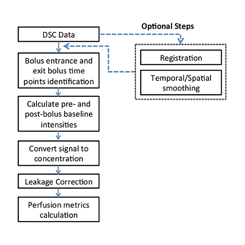
Calculating imaging biomarkers from perfusion signal time curves involves several steps; Figure 1 depicts the most commonly used steps. MRI perfusion imaging is capable of estimating the volume of blood that passes through the capillary bed per unit of time. The quantification can be performed in a relative or absolute manner. Although absolute quantification is preferable, it is much more challenging to perform in clinical practice due to many potential imaging and data processing artifacts. Thus, DSC typically produces images that are visually reviewed, and any measurements are expressed as a ratio to normal-appearing white matter. Relative cerebral blood volume (rCBV) measurements have been shown to correlate with tumor grade and histologic findings of increased tumor vascularity.⁸ They have also been shown to be useful in differentiating between progression and pseudo progression.^9,10 However, the selection of the reference region of interest (ROI) still remains an open issue in both clinical practice and longitudinal studies.¹¹

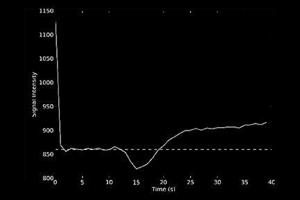
After the data are acquired, the baseline is defined; this often includes removal of the first 3 time points due to saturation effects. The start and end points of the bolus are calculated. Subsequently, the baseline signal intensity is calculated and the signal-time curves are converted to concentration-time curves. This is done for each voxel in the imaging volume. The rCBV image is the most important of the perfusion images for analyzing brain tumors and is computed by integrating the area under the time-concentration curve.¹² Some additional image types that can be computed include percent signal recovery, a measure of tumor leakiness; time to peak; bolus start and end time; and mean transit time. The latter two measures are frequently used in stroke imaging, but are of limited value in tumors.

Qualitative assessment

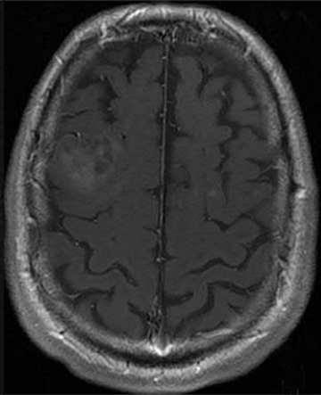
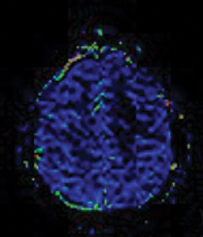
Several commercial software packages are available for calculating parametric maps like CBV from DSC-MRI. For routine clinical practice, visually inspecting the color maps can help to detect normal versus abnormal regions (Figure 2). This kind of assessment can be very useful in the clinical setting, but it depends on the windowing technique parameters used to present the data.

BBB disruption and leakage correction

One of the main challenges of DSC-MRI data analysis is contrast-agent extravasation due to BBB disruption. Figure 3 demonstrates the effect of this phenomenon on time-intensity curves. Instead of returning to baseline, the signal returns to a point higher than the initial baseline due to T1 effects, resulting in underestimation of the integration area. However, depending on the pulse sequence used, T2 or T2* leakage effects can predominate, resulting in overestimation of the rCBV value.¹²

The sequence type and parameters can affect how the concentration-time curves are distorted. A one-dimensional leakage simulation study performed by Quarles et al¹³ demonstrated that when T1 effects were removed, such as with the use of a dual-/multi-echo sequence, the measured transverse relaxation-rate-time course overestimated the true transverse relaxation–rate-time course. Therefore, the CBV would be overestimated. When T1 effects dominated (eg, when high flip angle and short repetition time were used), the measured transverse relaxation-rate-time course underestimated the true transverse relaxation-rate-time course; thus, the CBV would be underestimated.¹⁴

One technique is to minimize the contrast leakage effect by administering a contrast agent before acquiring the DSC images (referred to as ‘preloading’). However, animal studies suggest preloading is not very effective.¹⁵ The more popular and effective method is to apply mathematical models of the leakage during DSC data analysis.¹⁶ Figure 4 depicts an example of uncorrected and corrected CBV maps as well as the K2 image, a byproduct of the mathematical correction process. K2 refers to the leakage rate detected during DSC tumor imaging.

Spin echo vs gradient echo

Just as gradient-echo (GE) and spin-echo (SE) techniques can produce anatomical images, both GE and SE echo planar images (EPI) can be used for DSC-MRI. GE-DSC sequences tend to be more sensitive to larger vessels, such as veins, while SE-DSC techniques tend to show greater sensitivity to smaller vessels (capillaries) that should be more specific for tumor vessels.¹⁷ In actual practice, it appears that the vessels in tumors are large enough that GE imaging better demonstrates tumor vessels than SE imaging. However, imaging patients with GE sequences can be challenging after surgery because hemorrhage or metallic foreign bodies can produce signal loss and artifact.

Recently, a combination of the two techniques has been emerging, since it can provide simultaneous perfusion and permeability measurements.^18,19 These are referred to as a spin- and gradient-echo echo-planar imaging (SAGE EPI) MRI.

3T vs 1.5T

Transitioning DSC perfusion imaging from 1.5T to 3T creates a proportional increase in magnetic susceptibility. Practically, this means a higher signal-to-noise ratio (SNR) for a given dose of contrast²⁰ or that less contrast can be used in patients with limited renal function. 3T imaging’s increased sensitivity to contrast enhancement is well known. The correlate is that increased field strength leads to greater enhancement of T2 effect compared to 1.5T (the post-bolus baseline returned to a level above the baseline),²¹ also resulting in a higher SNR in CBV images. Because of the increased T1 effects at higher field, leakage is underestimated.²² Thus, field strength should be taken into account when comparing rCBV maps acquired at different field strengths.

Diffusion imaging: How it works

Due to their thermal energy, water molecules in tissue undergo a continuous random motion referred to as Brownian motion. While diffusion technically refers to the movement or transport of some substance without bulk motion within a medium like water, it also refers to the motion of water that occurs without bulk motion. Because water spins will run into constituents of cells, and because those cellular components have different concentrations in different parts, they will spread at different rates and not behave in the same way when moving in different directions.²³ For example, the membranes of cells restrict diffusion, and in acute stroke, where cells are not able to pump out enough water, the water that is present sees greater diffusion restriction because the interior of the cell has many more membranes and restricting structures than does the extracellular space.

The basic idea behind diffusion imaging is to use paired magnetic-field gradients to “encode,” and subsequently decode, the spatial motion of the molecules. Signal intensity is represented by the following equation:

S=S_0*exp⁡(-b*ADC) (Eq. 1)

In this equation, ADC is the apparent diffusion coefficient and b is the gradient factor commonly referred to as the b-factor. Sensitivity to diffusion-based contrast is controlled primarily by the b value. S_0 is the signal intensity when no diffusion gradients are used. The apparent diffusion coefficient is an average of the diffusion process occurring in the tissues. Qualitatively, Eq.1 means that the measured signal is reduced when diffusion gradients (b≠0) are applied.

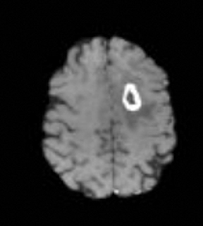
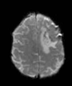
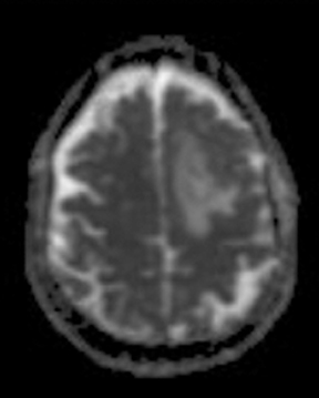
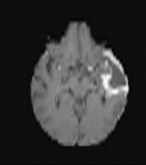
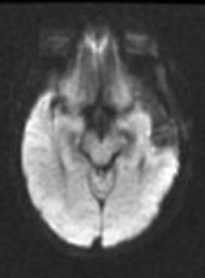
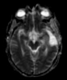
As the diffusing spins move inside the field, they are affected differently by the field; thus, their alignment with each other is destroyed. Since the measured signal is a summation of tiny signals from all individual spins, the misalignment, or “dephasing,” caused by the gradient pulses results in a drop in signal intensity; the longer the diffusion distance, the greater the signal loss. Based on Eq.1, for a fixed b-factor, high ADC values translate to low signal. A parametric ADC map (commonly referred to simply as an ADC map) can be generated after the application of different b-values as well as one image with no b-weighting (often referred to as the ‘b0 image’). The b-value is a factor in diffusion-weighted sequences. The b-factor summarizes the influence of the gradients on the diffusion-weighted images. Image intensities in the ADC map correspond to diffusion strength in the pixels.²³ Figure 5 depicts an ADC map and the images corresponding to two different b-values, as well as the corresponding T1 postcontrast image.

Although typical diffusion images have a spatial resolution of a few millimeters, they reflect events happening at the molecular level. As noted previously, when diffusing spins run into cellular constituents and membranes, the ADC value will be reduced when compared with diffusion in bulk water like cerebrospinal fluid (CSF).²⁴ Diffusion measurements become more complex when the structures restricting water diffusion have a structure themselves. For instance, axons restrict water diffusion perpendicular to their long axis, but not in the direction of the axon. This difference in magnitude of diffusion in different directions is referred to as diffusion anisotropy. What makes this more complex is that unless the axon is aligned with the imaging gradient, the reduction in signal will be seen in all 3 directions. When diffusion is to be measured in an anisotropic environment, diffusion tensor imaging is needed for a complete description.

Tumor cells are known to have many more membranes that both restrict motion and displace structures like axons that tend to have higher anisotropy. For that reason, there is great interest in using diffusion imaging in brain tumors. ADC has been found to correlate with tumor cellularity^25,26 and tumor grade,^27,28 with high-grade tumors having high cellular density and decreased ADC. Overlap in ADC values in high-grade tumors and low-grade tumors, however, has also been reported.²⁵ ADC values have been reported to predict responsiveness of temozolomide-refractory malignant glioma to bevacizumab treatment.²⁹

Studies^30-32 also indicate that recurrent tumors have lower ADC values than pseudoprogression, likely reflecting less water diffusion when there are many cells and cell membranes vs necrotic tissue or edema, where water is more able to diffuse. Finally, tumors in patients treated with anti-angiogenic agents often have reduced contrast enhancement, even when the tumor is progressing (referred to as pseudoresponse). ADC images appear to help detect this phenomenon. If one sees an enlarging area of low ADC values in a patient being treated with anti-angiogenic agents, tumor pseudoresponse should be considered.

Qualitative assessment

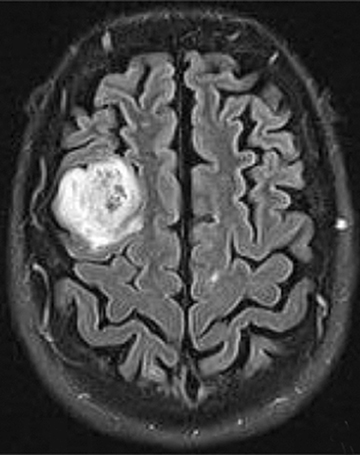
Diffusion imaging can be visually analyzed to identify underlying pathology (Figure 6). For the clinically used b-values, white and gray matter have similar ADC values, while a tumor takes a range of ADC values. As one would expect, cellular areas of tumors have low signal on ADC maps due to restricted diffusion. An inverse relationship between ADC values and tumor grade has been reported in the literature.³³ The destruction of cell membranes in necrotic brain lesions allows for virtually unhindered diffusion, yielding areas of elevated ADC values. Thus, areas of necrosis can be detected as elevated ADC within the tumor lesion.³⁴ However, the coarse resolution of diffusion MRI restricts detection of small areas of necrosis.³⁵ Very high diffusion values in peritumoral edema of high-grade gliomas may reflect fluid leakage into the extracellular space and destruction of the extracellular matrix ultra-structure by malignant cell infiltration.³⁶

Quantitative assessment

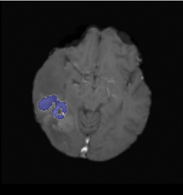
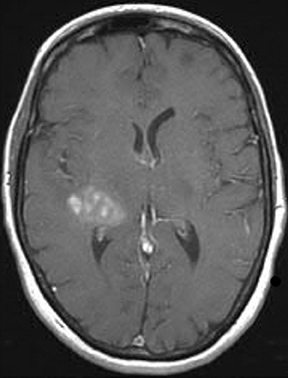
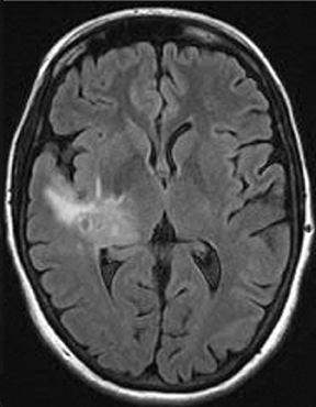
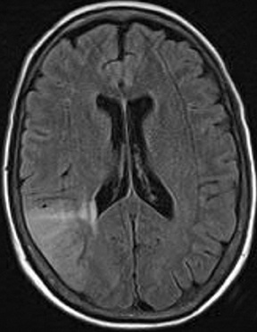
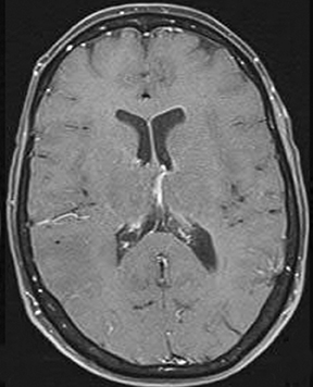
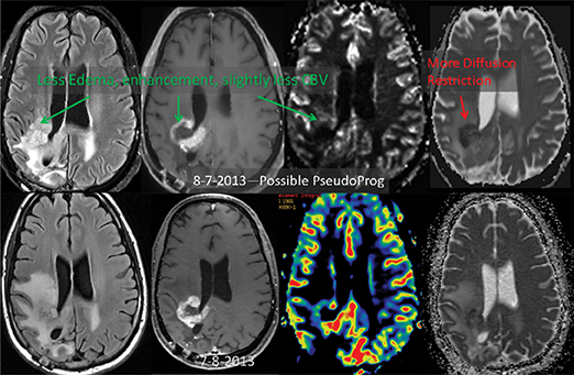
ADC maps can provide additional information for tumor grading and assessing the effects of therapy in cases where T1- and T2-weighted images alone provide insufficient diagnostic information.³⁵ Histogram analysis based on the ADC of the enhancing tumor has been reported to assist in differentiating true progression from pseudoprogression in glioblastomas.^37,38 However, biomarkers such as percentile values of the cumulative ADC histogram must also be investigated. In differentiating between progression and pseudoprogression, the underlying hypothesis is that the part of the histogram corresponding to lower values is related to the viable component of the tumor, while the higher part is related to edematous/necrotic tissue.³⁹ This approach is adapted to the heterogeneous nature of tumors that include areas of active tumor and necrotic or “dying” portions. An example of pseudoprogression with an enlarging region of low ADC is shown in Figure 7.

There is also interest in studying components immediately adjacent to the contrast-enhancing portion of the tumor (which traditionally has been the focus). In this case, the tumor is subdivided into three layers (central core, peripheral enhancement, and peritumoral layer), and the tumor status is determined according to the pattern of values in the three layers.⁴⁰

Additionally, monitoring the differences in ADC values (capturing fluid-volume changes in intra- and extracellular compartments) of the enhancing regions during post-therapy imaging has the potential to differentiate radiation effects from tumor recurrence or progression.³⁰

Choosing a b-value

White and gray matter exhibit very similar ADC values, while different tumor types have been observed to exhibit dissimilar diffusion values³⁵ for typically employed b-values. A b-factor around 1000 is the most commonly utilized value for brain imaging in clinical and research settings. This value has been shown to be sensitive to detecting and delineating restricted diffusion since it provides the best tradeoff between signal attenuation from diffusion and background noise.⁴¹

ADC maps created with larger b-values, however, have been reported to better differentiate progression from pseudoprogression³⁸ and to correlate with microstructure. Diffusion imaging with a higher b-value yields better contrast and less T2 shine-through effect⁴² than reduced SNR, leading to longer acquisition times and, therefore more motion artifacts.⁴³

A limited number of studies have compared multiple imaging approaches to explore therapy outcome. However, the value of combining rCBV- and ADC-based biomarkers has been recognized in several papers.⁴⁰ For instance, increased rCBV values and decreased ADCs appear to help separate true progression from pseudoprogression.

A challenge to clinical implementation of DSC-MRI-based biomarkers is the lack of standardized approaches to data acquisition, measurement, and analysis,²⁴ with resulting decreased reproducibility. Accurate CBV quantification is difficult, especially in cases of glioblastoma (GBM) where the BBB has been interrupted and contrast leakage occurs. Perfusion-analysis software is widely available in clinical practice; however, it is often treated as a black box tool. Some of this software incorporates mathematical techniques to deal with contrast agent leakage. The values produced are generally accepted, but validation is challenging.

Assessing the accuracy and reliability of leakage-correction methods can be achieved only with an appropriate phantom. However, creating a phantom that accurately reflects biology is very difficult, if not impossible; development of digital phantoms that simulate contrast extravasation remains an open research issue.

The rCBV thresholds for differentiating progression vs pseudoprogression or tumor grading are often not the same across different perfusion-analysis software packages because different software packages utilize different methodologies for estimating bolus entrance and exit times, and determining baselines, model fitting, integration methods, and mathematical models to correct for contrast-agent extravasation.

Most approaches to measuring rCBV use a normal-appearing region in contralateral white matter as a control region; however, no standardized criteria exist on how these regions of interest (ROI) are chosen. To reduce variability in rCBV measurements, ROI selection must also be standardized.

Tumor ROI selection delineation is also critical; areas of necrosis must be excluded from analyses of tumor ADCs or CBV. Necrotic regions are common in high-grade tumors, and in ADC analysis, for example, they can contribute to raising the mean ADC values of the tumor. Necrotic areas are also known to have contrast enhancement, making ROI determination very challenging. Furthermore, when defining ROIs using T1 images aligning the T1 images with the diffusion or perfusion images is necessary, but not always straightforward.

Conclusions

DSC-MRI perfusion and diffusion MRI have already contributed to our understanding of brain tumors and the effects of therapy. The key points are that rCBV images can give strong indications that a tumor may be of a higher grade than contrast images might suggest; rCBV images can help to distinguish treatment effects from true tumor progression; and ADC images can be helpful when interpreting images of patients treated with anti-angiogenic agents. Much still remains to be learned about these imaging methods for brain tumors, and investigation is required to define their role in everyday clinical practice and clinical trials.

REFERENCES

1. Wen PY, Macdonald DR, Reardon DA, et al. Updated response assessment criteria for high-grade gliomas: Response assessment in neuro-oncology working group. J Clin Oncol 2010;28:1963-1972.
2. Macdonald DR, Cascino TL, Schold SC, Jr., et al. Response criteria for phase II studies of supratentorial malignant glioma. J Clin Oncol. 1990;8:1277-1280.
3. Provenzale JM, Mukundan S, Barboriak DP. Diffusion-weighted and perfusion MR imaging for brain tumor characterization and assessment of treatment response. Radiology. 2006;239:632-649.
4. Brandao LA, Shiroishi MS, Law M. BrainTumors. A multimodality approach with diffusion-weighted imaging, diffusion tensor imaging, magnetic resonance spectroscopy, dynamic susceptibility contrast and dynamic contrast-enhanced magnetic resonance imaging. Magn Reson Imaging Clin N Am. 2013;21:199-239.
5. Rosen BR, Belliveau JW, Vevea JM, et al. Perfusion imaging with NMR contrast agents. Magn Reson Med.1990;14:249-265.
6. Walker C, Baborie A, Crooks D, et al. Biology, genetics and imaging of glial cell tumours. Br J Radiol. 2011;84 Spec No 2:S90-106.
7. Jain RK, di Tomaso E, Duda DG, et al. Angiogenesis in brain tumours. Nat Rev Neurosci. 2007; 8:610-622.
8. Law M, Yang S, Wang H, et al. Glioma grading: Sensitivity, specificity, and predictive values of perfusion MR imaging and proton MR spectroscopic imaging compared with conventional MR imaging. AJNR Am J Neuroradiol. 2003;24:1989-1998.
9. Hu LS, Eschbacher JM, Heiserman JE, et al. Reevaluating the imaging definition of tumor progression: Perfusion MRI quantifies recurrent glioblastoma tumor fraction, pseudoprogression, and radiation necrosis to predict survival. Neuro Oncol. 2012;14:919-930.
10. Essig M, Shiroishi MS, Nguyen TB, et al. Perfusion MRI: The five most frequently asked technical questions. AJR Am J Roentgenol. 2013;200:24-34.
11. Bedekar D, Jensen T, Schmainda KM. Standardization of relative cerebral blood volume (rCBV) image maps for ease of both inter- and intrapatient comparisons. Magn Reson Med. 2010;64:907-913.
12. Paulson ES, Schmainda KM. Comparison of dynamic susceptibility-weighted contrast-enhanced MR methods: Recommendations for measuring relative cerebral blood volume in brain tumors. Radiology. 2008;249:601-613.
13. Quarles CC, Gochberg DF, Gore JC, et al. A theoretical framework to model DSC-MRI data acquired in the presence of contrast agent extravasation. Phys Med Biol. 2009;54:5749-5766.
14. . Willats L, Calamante F. The 39 steps: Evading error and deciphering the secrets for accurate dynamic susceptibility contrast MRI. NMR Biomed. 2013;26:913-931.
15. Gahramanov S, Muldoon LL, Li X, et al. Improved perfusion MR imaging assessment of intracerebral tumor blood volume and antiangiogenic therapy efficacy in a rat model with Ferumoxytol. Radiology. 2011;261:796-804.
16. . Boxerman JL, Schmainda KM, Weisskoff RM. Relative cerebral blood volume maps corrected for contrast agent extravasation significantly correlate with glioma tumor grade, whereas uncorrected maps do not. AJNR Am J Neuroradiol. 2006;27:859-867.
17. . Speck O, Chang L, DeSilva NM, et al. Perfusion MRI of the human brain with dynamic susceptibility contrast: Gradient-echo versus spin-echo techniques. J Magn ResonImaging. 2000;12:381-387.
18. Schmiedeskamp H, Andre JB, Straka M, et al. Simultaneous perfusion and permeability measurements using combined spin- and gradient-echo MRI. J Cereb Blood Flow Metab. 2013;33:732-743.
19. . Schmiedeskamp H, Straka M, Newbould RD, et al. Combined spin- and gradient-echo perfusion-weighted imaging. Magn Reson Med. 2012;68: 30-40.
20. Alvarez-Linera J. 3T MRI: Advances in brain imaging. Eur J Radiol. 2008;67:415-426.
21. Liu HL, Wu YY, Yang WS, et al. Is Weisskoff model valid for the correction of contrast agent extravasation with combined T-1 and T-2* effects in dynamic susceptibility contrast MRI? Med Phys. 2011;38:802-809.
22. Mauz N, Krainik A, Tropres I, et al. Perfusion magnetic resonance imaging: Comparison of semiologic characteristics in first-pass perfusion of brain tumors at 1.5 and 3 Tesla. J Neuroradiol. 2012;39:308-316.
23. Hagmann P, Jonasson L, Maeder P, et al. Understanding diffusion MR imaging techniques: From scalar diffusion-weighted imaging to diffusion tensor imaging and beyond. Radiographics. 2006;26 Suppl 1:S205-223.
24. Padhani AR, Liu G, Koh DM, et al. Diffusion-weighted magnetic resonance imaging as a cancer biomarker: Consensus and recommendations. Neoplasia. 2009;11:102-125.
25. Kono K, Inoue Y, Nakayama K, et al. The role of diffusion-weighted imaging in patients with brain tumors. AJNR Am J Neuroradiol. 2001;22: 1081-1088.
26. Stadnik TW, Demaerel P, Luypaert RR, et al. Imaging tutorial: Differential diagnosis of bright lesions on diffusion-weighted MR images. Radiographics. 2003;23:e7.
27. Bulakbasi N, Kocaoglu M, Ors F, et al. Combination of single-voxel proton MR spectroscopy and apparent diffusion coefficient calculation in the evaluation of common brain tumors. AJNR Am J Neuroradiol. 2003;24:225-233.
28. Yamasaki F, Kurisu K, Satoh K, et al. Apparent diffusion coefficient of human brain tumors at MR imaging. Radiology. 2005;235:985-991.
29. Nagane M, Kobayashi K, Tanaka M, et al. Predictive significance of mean apparent diffusion coefficient value for responsiveness of temozolomide-refractory malignant glioma to bevacizumab: Preliminary report. Int J Clin Oncol. 2013; [Epub ahead of print].
30. Hein PA, Eskey CJ, Dunn JF, et al. Diffusion-weighted imaging in the follow-up of treated high-grade gliomas: Tumor recurrence versus radiation injury. AJNR Am J Neuroradiol. 2004;25:201-209.
31. Lee WJ, Choi SH, Park CK, et al. Diffusion-weighted MR imaging for the differentiation of true progression from pseudoprogression following concomitant radiotherapy with temozolomide in patients with newly diagnosed high-grade gliomas. Acad Radiol. 2012;19:1353-1361.
32. Zeng QS, Li CF, Liu H, Z,et al. Distinction between recurrent glioma and radiation injury using magnetic resonance spectroscopy in combination with diffusion-weighted imaging. Int J Radiat Oncol Biol Phys. 2007;68:151-158.
33. Hayashida Y, Hirai T, Morishita S, et al. Diffusion-weighted imaging of metastatic brain tumors: Comparison with histologic type and tumor cellularity. AJNR Am J Neuroradiol. 2006;27:1419-1425.
34. Lyng H, Haraldseth O, Rofstad EK. Measurement of cell density and necrotic fraction in human melanoma xenografts by diffusion weighted magnetic resonance imaging. Magn Reson Med. 2000;43:828-836.
35. Maier SE, Sun Y, Mulkern RV. Diffusion imaging of brain tumors. NMR Biomed. 2010;23:849-864.
36. Morita KI, Matsuzawa H, Fujii Y, et al. Diffusion tensor analysis of peritumoral edema using lambda chart analysis indicative of the heterogeneity of the microstructure within edema. J Neurosurg. 2005;102:336-341.
37. Pope WB, Qiao XJ, Kim HJ, et al. Apparent diffusion coefficient histogram analysis stratifies progression-free and overall survival in patients with recurrent GBM treated with bevacizumab: A multi-center study. J Neurooncol. 2012;108:491-498.
38. Chu HH, Choi SH, Ryoo I, et al. Differentiation of true progression from pseudoprogression in glioblastoma treated with radiation therapy and concomitant temozolomide: Comparison study of standard and high-b-value diffusion-weighted imaging. Radiology. [Epub ahead of print Jun 14, 2013].
39. Pope WB, Qiao XJ, Kim HJ, et al. Apparent diffusion coefficient histogram analysis stratifies progression-free and overall survival in patients with recurrent GBM treated with bevacizumab: A multi-center study. J Neurooncol. 2012;108:491-498.
40. Cha J, Kim ST, Kim HJ, et al. Analysis of the layering pattern of the apparent diffusion coefficient (ADC) for differentiation of radiation necrosis from tumour progression. Eur Radiol. 2013;23:879-886.
41. Xing D, Papadakis NG, Huang CL, et al. Optimised diffusion-weighting for measurement of apparent diffusion coefficient (ADC) in human brain. Magn Reson Imaging. 1997;15:771-784.
42. Burdette JH, Durden DD, Elster AD, et al. High b-value diffusion-weighted MRI of normal brain. J Comput Assist Tomogr. 2001;25:515-519.
43. Ben-Amitay S, Jones DK, Assaf Y. Motion correction and registration of high b-value diffusion weighted images. Magn Reson Med. 2012;67:1694-1702.